27.10
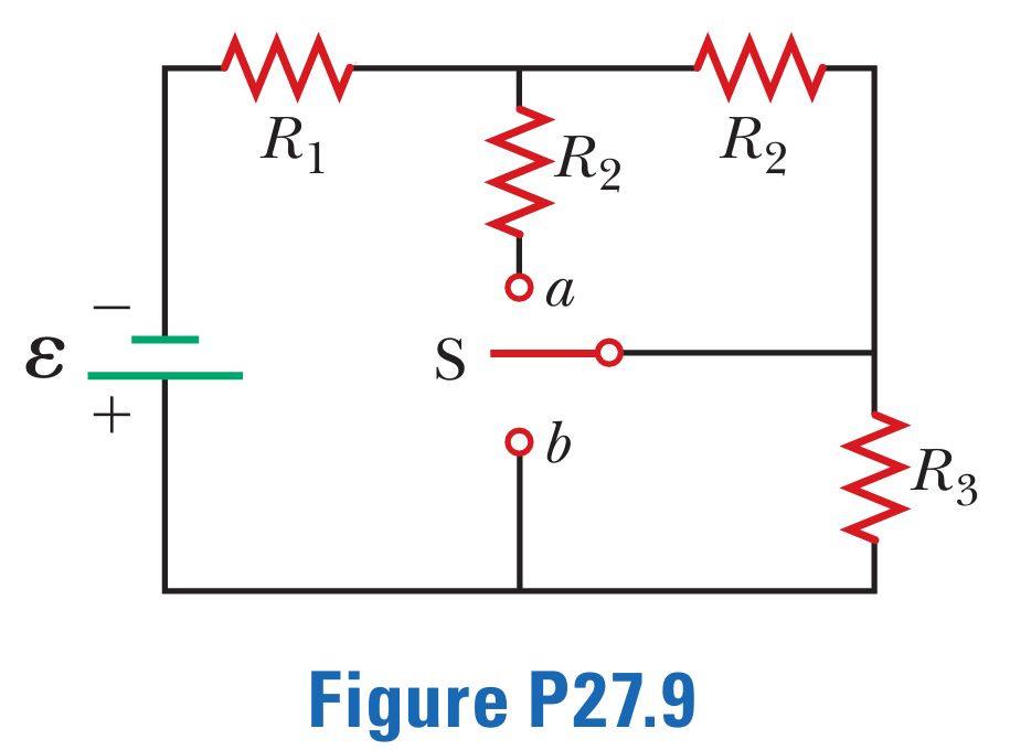
A battery with emf \(\varepsilon \) and no internal resistance supplies current to the circuit shown in Figure P27.9. When the double-throw switch S is open as shown in the figure, the current in the battery is I0 . When the switch is closed in position a, the current in the battery is Ia . When the switch is closed in position b, the current in the battery is Ib . Find the resistances (a) R1 , (b) R2 , and (c) R3 .
Solution
Case 1: When Disconnected
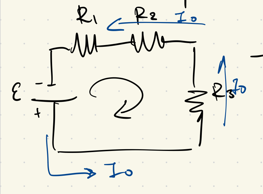
\[ \hspace{1pt} - \mathcal{E} + I_0 R_1 + I_0 R_2 + I_0 R_3 = 0 \]
\[ \Rightarrow - \mathcal{E} + I_0 (R_1 + R_2 + R_3) = 0 \tag{1} \]
Case 2: Connected at Point a
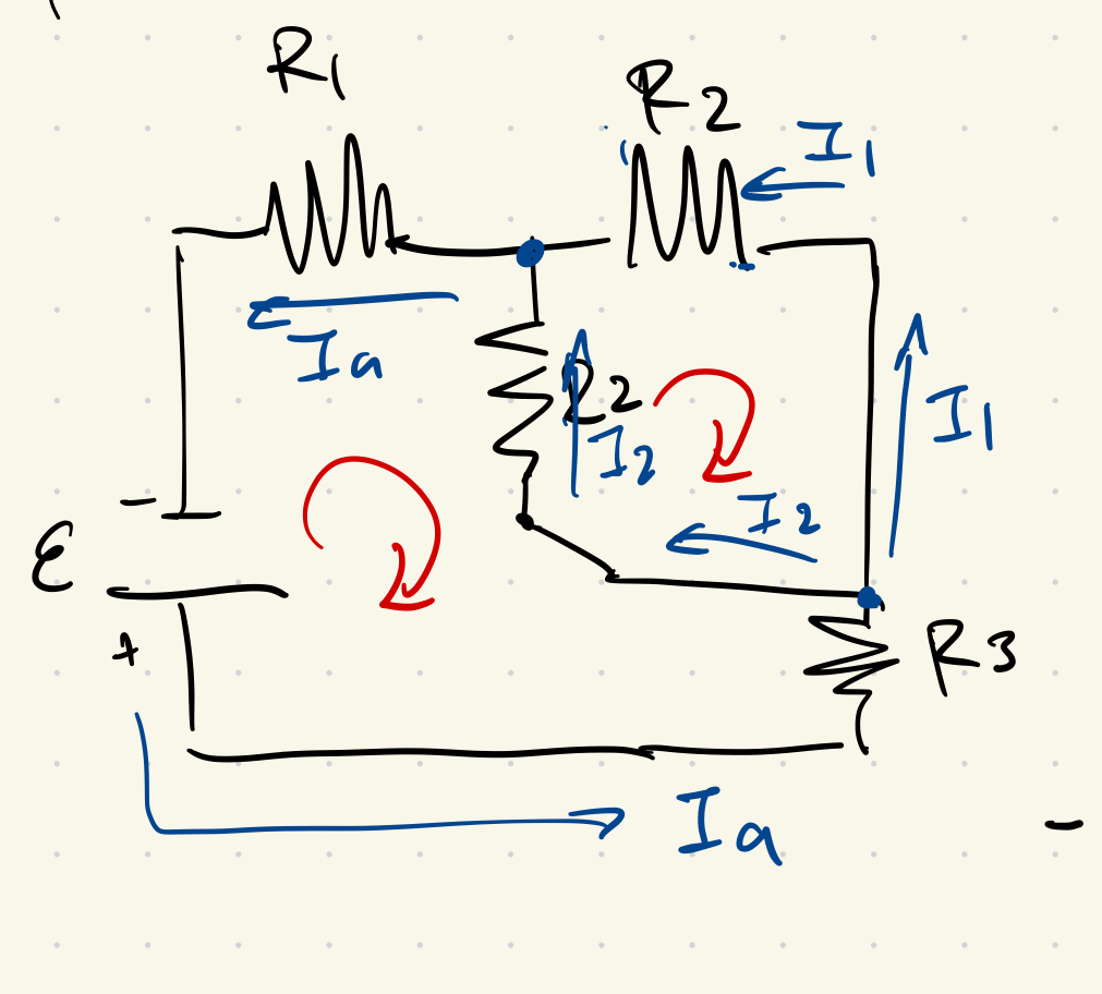
From node analysis:
\[ I_a - I_1 - I_2 = 0 \]
Loop 1:
\[ \hspace{1pt} - \mathcal{E} + R_1 I_a + R_2 I_2 + R_3 I_a = 0 \]
\[ \hspace{1pt} - \mathcal{E} + R_2 I_2 + (R_1 + R_3) I_a = 0 \tag{A} \]
Loop 2:
From the right-hand vertical branch:
\[ R_2 I_2 = R_2 I_1 \quad \Rightarrow \quad I_2 = I_1 \]
Substitute into node equation:
\[ I_a = 2 I_1 = 2 I_2 \]
Substitute into (A):
\[ \hspace{1pt} - \mathcal{E} + R_2 \cdot \frac{I_a}{2} + (R_1 + R_3) I_a = 0 \]
\[ \hspace{1pt} - \mathcal{E} + I_a \left( \frac{R_2}{2} + R_1 + R_3 \right) = 0 \tag{2} \]
Case 3: Connected at Point b
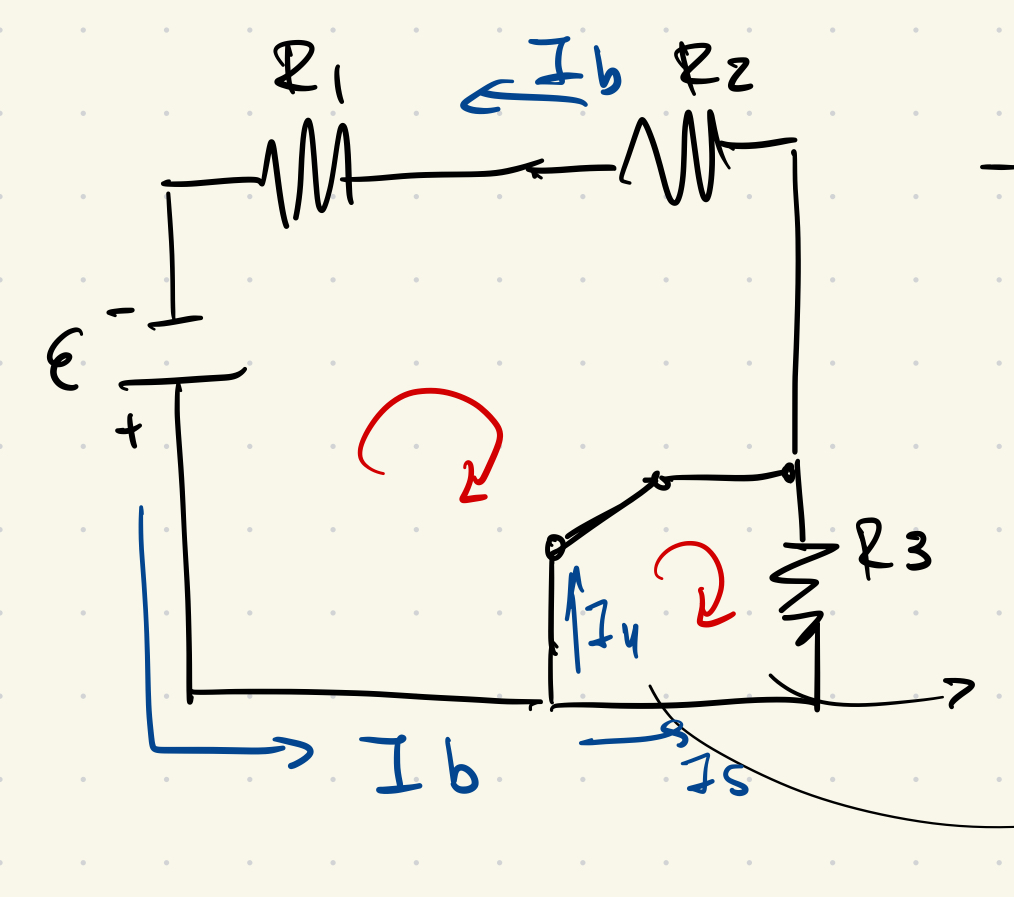
From the loop:
\[ \hspace{1pt} - \mathcal{E} + I_b (R_1 + R_2) = 0 \tag{3} \]
For the shorted R₃ branch: \( I_5 R_3 = 0 \), so \( I_5 = 0 \), it doesn’t affect the rest of the circuit.
From equation (2):
\[ \hspace{1pt} -\mathcal{E} + I_a \left( \frac{R_2}{2} + R_1 + R_3 \right) = 0 \]
Solve for ( R_3 ):
\[ \hspace{1pt} -I_a R_3 = -\mathcal{E} + I_a \left( \frac{R_2}{2} + R_1 \right) \]
\[ \Rightarrow R_3 = \frac{\mathcal{E}}{I_a} - \frac{R_2}{2} - R_1 \]
Substitute into equation (1):
\[ \hspace{1pt} -\mathcal{E} + I_0 \left( R_1 + R_2 + \left( \frac{\mathcal{E}}{I_a} - \frac{R_2}{2} - R_1 \right) \right) = 0 \]
\[ \hspace{1pt} - \mathcal{E} + I_0 \left( \frac{R_2}{2} + \frac{\mathcal{E}}{I_a} \right) = 0 \]
\[ \hspace{1pt} - \mathcal{E} \left( 1 - \frac{I_0}{I_a} \right) + \frac{R_2}{2} I_0 = 0 \tag{★} \]
From (3):
\[ \Rightarrow R_2 = \frac{\mathcal{E}}{I_b} - R_1 \]
Replacing in ★:
\[ \hspace{1pt} - \mathcal{E} \left( 1 - \frac{I_0}{I_a} \right) + \frac{I_0}{2} \left( \frac{\mathcal{E}}{I_b} - R_1 \right) = 0 \]
Solving for (R_1) yields:
\[ \boxed{ R_1 = \mathcal{E} \left( -\frac{2}{I_0} + \frac{2}{I_a} + \frac{1}{I_b} \right) } \]
Substitute into ( R_2 ):
\[ R_2 = \frac{\mathcal{E}}{I_b} - \mathcal{E} \left( -\frac{2}{I_0} + \frac{2}{I_a} + \frac{1}{I_b} \right) \]
\[ R_2 = \mathcal{E} \left( \frac{1}{I_b} + \frac{2}{I_0} - \frac{2}{I_a} - \frac{1}{I_b} \right) \]
\[ \Rightarrow R_2 = 2\mathcal{E} \left( \frac{1}{I_0} - \frac{1}{I_a} \right) \]
\[ \boxed{ R_2 = 2\mathcal{E} \left( \frac{1}{I_0} - \frac{1}{I_a} \right) } \]
Finally, Solve for ( R_3 )
\[ R_3 = \frac{\mathcal{E}}{I_a} - \frac{R_2}{2} - R_1 \]
Substitute the expressions for ( R_2 ) and ( R_1 ):
\[ R_3 = \frac{\mathcal{E}}{I_a} - \mathcal{E} \left( \frac{1}{I_0} - \frac{1}{I_a} \right) - \mathcal{E} \left( -\frac{2}{I_0} + \frac{2}{I_a} + \frac{1}{I_b} \right) \]
Simplify:
\[ R_3 = \mathcal{E} \left( \frac{1}{I_a} - \frac{1}{I_0} + \frac{1}{I_a} + \frac{2}{I_0} - \frac{2}{I_a} - \frac{1}{I_b} \right) \]
\[ \Rightarrow \boxed{ R_3 = \mathcal{E} \left( \frac{1}{I_0} - \frac{1}{I_b} \right) } \]